The MPC and MPS

• Intro

  • When investment spending increases, there will be an increase in the income and the value of aggregate output by the same amount

  • An increase in aggregate output leads to an increase in disposable income and to more consumer spending, which leads to increased output

  • How large is the total effect on aggregate output if we sum up all the rounds of spending increases

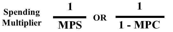
  • It depends on what economists called the marginal propensity to consume (MPC) or the marginal propensity to save (MPS)

  • $\text{MPS} = \dfrac{\text{Change in savings}}{\text{Change in income}}$

  • $\text{MPC} = \dfrac{\text{Change in consumption}}{\text{Change in income}}$

  • MPC + MPS = 1

• The marginal Propensity to Consume

  • The MPC is a number between 0 and 1

  • If consumers save all their money, the number would be 0

  • If consumers spend all their money, the number would be 1

  • Usually, the number is between 0 and 1 with industrialized countries having a higher number and developing countries with lower numbers

  • If the MPC is 0.8, what's the impact on the total aggregate spending if there's an increase of 50 million in spending?

    • Total Increase = Spending Multiplier * Initial Increase = 1/(1-0.8) * 50 = 250

The Multiplier Effect

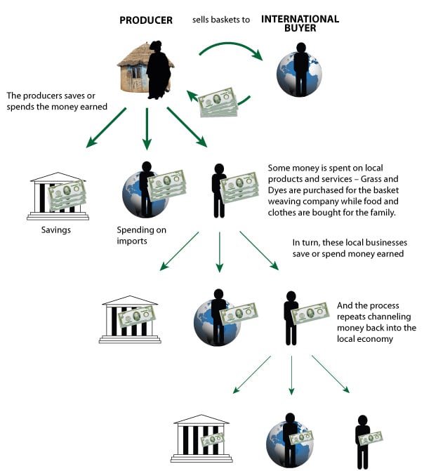
• Autonomous change in aggregate spending

  • an initial rise or fall in aggregate spending that is the cause, not the result, of a series of income and spending changes

• Multiplier

  • ratio of the total change in real GDP caused by an autonomous change in aggregate spending to the size of that autonomous change

  

• The size of the multiplier depends on the MPC

  • The higher the MPC, the more disposable income get recycled back into consumer spending

  • The lower the MPC, the more disposable income "leak out" into savings

Consumption Function

• Consumption function is an equation showing how an individual household's consumer spending changes with disposable income

• Autonomous consumer spending would be the amount spent regardless of income

  

  

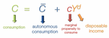
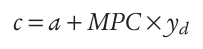
• Let's assume that a equals $20,000 and the MPC equals 0.6. What would the consumption be if the income is $100,000? $200,000?

  • c = a + MPC * y_d = 20,000 + 0.6 * 100,000 = 80,000

  • c = a + MPC * y_d = 20,000 + 0.6 * 200,000 = 140,000

• Graph

  

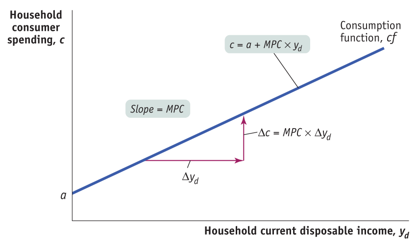
Shift of the Aggregate Consumption Function

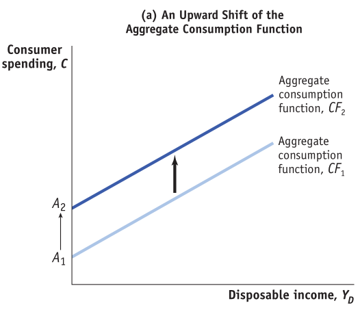
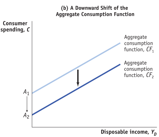
• Changes in Expected Future Disposable Income

  • If you land a higher-paying job, you will tend to consume more money now even though your current income is the same

  • Conversely, if you are worried about a job layoff, you will probably decrease your current expense.

• Changes in Aggregate Wealth

  • A booming stock market will tend to increase an individual's wealth, and therefore, his consumption

  • A fall in housing prices, conversely, will tend to decrease an individual's net worth, and therefore her consumption

Investment Spending

• Planned investment spending is the investment spending that businesses intend to undertake during a given time period

• If interest rates goes up, less investment spending occurs.

• If interest rates go down, there is more investment spending

• High expected future growth rate of GDP increases investment

• Low expected future growth rate decreases investment

• 

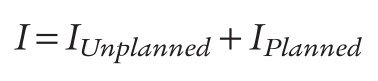
• Positive unplanned inventory investment occurs when sales are less than business expects. Excess sales leads to negative unplanned inventory investment

• Rising inventory indicates slowing economy

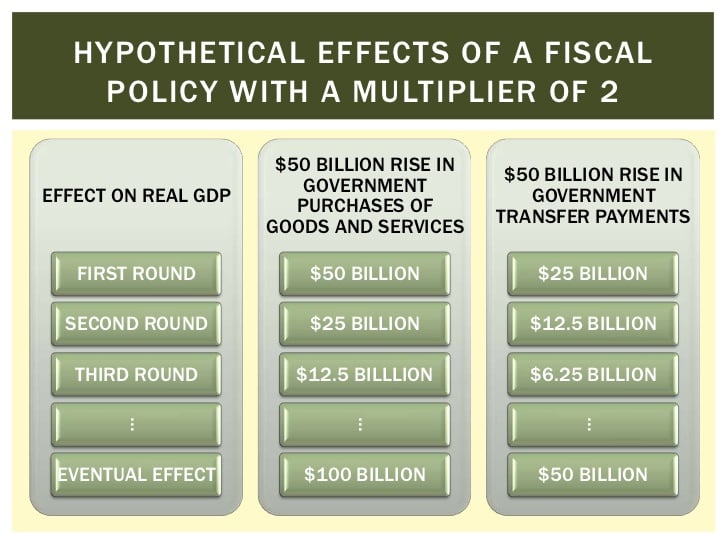
Tax (or Government Transfer) Multiplier

• Changes in taxes (or increase in transfer payment) shifts the aggregate demand curve by less than an equal-sized change in government purchases

• The presence of taxed decrease the multiplier

  

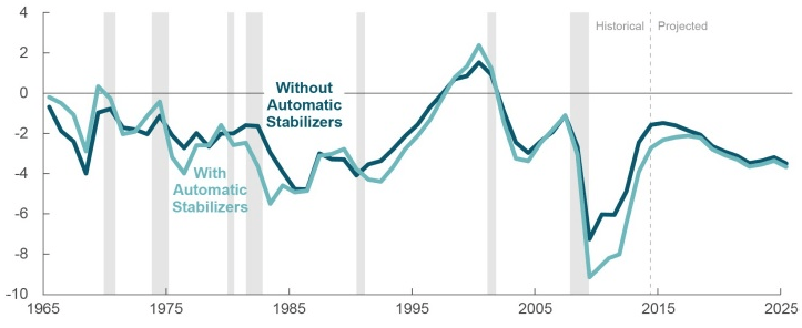
Automatic Stabilizers

• Government spending and taxation rules that cause fiscal policy to be automatically expansionary when the economy contracts and automatically contractionary when the economy expands

• As the economy expands, the multiplier reduces because the increase in income is siphoned off

• As the economy contracts, the multiplier increase because the government is collecting less in taxes (a de facto expansionary policy in the face of a recession)